Free energy from Coriolis pressure

Created by Zoltan Losonc (feprinciples@on.mailshell.com) on 14 November 2004. Last updated on 28 November 2004

Commentaires: Une traduction française sera ajoutée ultérieurement

Introduction

It is well known to free energy researchers that there are several alleged free energy devices, which utilize the inward and/or outward spiraling helical movement of fluid substances. Some of such devices are the inventions of Victor Schauberger, but the Clem turbine, and the hydro-electric power plant Rheinfelden on the high Rhine etc. also belong to the same category. In fact the Schauberger’s “Home Power Generator” shown in the book “The Energy Evolution” fig 34 has the same structure as the alleged Clem turbine, that is made of spirally arranged pipes fixed around a cone, ending in nozzles at the periphery.

Schauberger gave some quite exotic and (to me) not very convincing explanation about the basic principles that supposed to be responsible for the excess energy generation. His most rational points were centered around his claim that the inward spiraling (imploding) water cools down, and the lost heat energy is converted into kinetic energy (but how and why?). This however, does not explain the source of excess energy in devices like his mentioned Home Power Generator (in which the water appears to move downward and from the center towards the periphery in the spiral pipes), and in Clem turbine where the fluid does not follow an imploding path, but exactly the opposite.

The subject of this presentation is to show a possible fluid dynamic principle that can be responsible for the generation of excess energy. The principle is fairly simple, but in order to better understand its mechanism and implications let us start with a little exercise. Let us examine the energy balance of a simple lawn sprinkler that is basically the same as that of a revolving drum with water inlet at the shaft, and outlet through the tangentially arranged nozzles at the periphery.

The simplified analysis of an ideal lawn sprinkler

This sprinkler is made of a pipe that is fixed to a hollow shaft at its middle and has attached nozzles at both ends bent into tangential direction. The sprinkler (fig 1), rotates around the shaft counter clockwise, the water enters at the center through the hollow shaft and exits through the nozzles in clockwise (relative) direction. Let us examine an idealistic case when the angular velocity ω , and the radial velocity of the water v_r are constant, and neglecting friction resistance. There is a constant pressure p₀ at the center maintained by an external pump (not shown), and the pressure at the nozzle outlets are assumed to be zero.

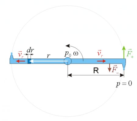
Fig 1.

We want to know the torque that the fluid exerts upon the sprinkler; the mechanical power of this torque; the relative and absolute velocity of the stream at the nozzle exit and its power content; and finally the power of the external pump. This way we will be able to evaluate the energy balance of the system.

The formula for the pressure p in a centrifuge as the function of radius r and density ρ has been demonstrated in the Appendix and it is:

In our case the radius of the inner water surface r₀ = 0, and we have an additional constant pressure component p₀ at the axis. Thus the formula for the centrifugal pressure valid in the sprinkler arms (but not in the nozzles) becomes:

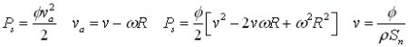
The relative tangential stream velocity v at the outlet of the nozzle is calculated as:

Where:

• v – relative stream velocity at the outlet;
• S_n – surface area of the nozzle’s outlet;
• S_p – the pipe’s cross-section area;
• R – radius to the nozzle’s center.

A special case:

If the cross section area of the nozzle outlet opening S_n is much smaller than the cross section area of the sprinkler arm S_p, then the relative outlet velocity v is much greater than the radial water velocity in the arms v_r. In such case v_r and S_n can be neglected in the above formulas. If we take the special case when p₀ = 0 and substitute the pressure then we get that:

This result shows that when the pump is not there (and p₀=0) then the water stream velocity v at the outlet relative to the rotating nozzle is the same as the absolute velocity of the nozzle v_n = ωR just in opposite direction. The absolute velocity of the outlet stream (relative to the stationary frame of reference) in this special case is v_a = v_n - v = ω R = ω R = 0.

We can make an interesting observation here, that no matter how fast (ω) we rotate the sprinkler, if the inlet pressure is the same as the pressure at the outlet, then the absolute outlet stream velocity is always zero, and consequently the kinetic energy of the stream is also zero. If the law of energy conservation is valid, then obviously we will be able to turn the sprinkler (theoretically) with arbitrarily high angular velocity without investing any mechanical work (without resistance) since no energy leaves the sprinkler. In this case the forward acting driving torque of the nozzle has the same magnitude as the braking Coriolis torque acting on the walls of the sprinkler arms, thus they cancel each other. This can be confirmed using the formulas below.

One more interesting conclusion can be made for this special frictionless case, namely that no matter how fast we may turn the sprinkler, the absolute tangential velocity of the outlet stream can never have identical direction with the nozzle. The absolute velocity of the stream is either zero or if p₀ then it has a direction opposite to the velocity of the nozzle. In practical cases when the friction resistance of the pipe is significant, or the inlet pressure is less than the outlet pressure then this rule is not valid anymore, and the stream may fly in the same direction as the nozzles.

The energy balance in general case:

Let us calculate the input power fed into the sprinkler. This is made up of the kinetic energy of the inlet stream and the flow work performed by the pump. The input kinetic energy flow is:

Where:

• Φ - is the mass flow;
• v _in – inlet stream velocity;
• V – volume;
• t - time

The power of the pump is:

The input power is:

The output power is made up of the mechanical work component of the resultant torque, and of the kinetic energy flow of the outlet water stream in stationary frame of reference. The positive torque M+ of the nozzle is (F – is force):

We have already mentioned that the driving torque of the nozzle is counteracted by the braking negative torque of the Coriolis force in the pipes. Let us calculate now this Coriolis torque. When a mass moves in radial direction in a rotating frame of reference then besides the centrifugal force, there will be an additional Coriolis force that will act on the mass. This force acts in tangential direction and when the mass moves outward then it brakes the rotation; when it moves inward (toward the axis) then it a tries to accelerate the rotation.

The Coriolis torque M- (see fig 1) on the sprinkler arm can be calculated by integrating the elementary torque components along the pipe arms that act on the infinitesimal fluid masses dm:

The resultant torque is the sum of the above positive and negative torque components:

The power of the resultant torque is:

The kinetic energy flow of the outlet water stream in stationary frame of reference is:

The total output power is the sum of these kinetic and mechanical powers:

Now we have both formulas necessary for calculating the energy balance of the sprinkler P_in and P_out. If we substitute some specific values in both these formulas then we will find that they produce always identical results P_in=P_out. Since the input power is always the same as the output power there is no excess energy, and the law of energy conservation is valid for the analyzed sprinkler.

Coriolis pressure as the source of excess energy

It is a well known phenomenon that if someone is placed into a rotating centrifuge he will feel a centrifugal force acting on his body, trying to move him away from the axis in radial direction. This force has similar effect as a gravitational force, and we may consider it as an artificial radially oriented ‘gravitational’ force field with an intensity of:

There is one more similar force that acts on the body in a rotating centrifuge that is called Coriolis force, but this is present only if the body of mass m moves in radial direction with velocity v_r (either towards the axis or away from the axis). This force acts on the body in tangential direction with a force of:

This force is perpendicular to the radial velocity component v_r and its direction is opposite to the rotation when the body moves away from the axis; but it has the same direction as the rotation if the body moves towards the axis. Since the nature of this Coriolis force field is similar to that of the centrifugal- and gravitational force fields, we can consider it as an additional artificial ‘gravitational’ force field in a rotating centrifuge, having an intensity of:

The shape of the centrifugal force field is radially oriented and divergent, whereas the shape of the Coriolis force lines are circular. One might get the first impression that if a body is left to be accelerated along these circular force lines, then it may be accelerated indefinitely and obtain enormous energy in the rotating frame of reference. But this is not possible because the Coriolis force field exists only if the body also moves in radial direction v_r and consequently it will follow a spiral path (fig 2).

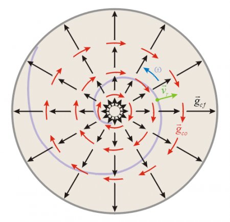
Fig 2.

What happens if some fluid is present in a gravitational force field, or such artificial force fields as the centrifugal- and Coriolis fields? It is well known that if a container is filled with a liquid then the gravitation will induce a pressure gradient in it. The pressure p will increase towards the bottom of the container (in the direction of the gravitational field) and its magnitude can be calculated as the product of the liquid density r , the gravitational acceleration g, and the height of the liquid column h: p=r *g*h.
It is important to note that this pressure is independent of the shape of the container, and this phenomenon is known in physics as the ‘hydrostatic paradox’.

The same phenomenon is also valid for the centrifugal- g_cf and Coriolis g_co fields of acceleration. That means, if a liquid is present in a rotating frame of reference (ex. in a centrifuge) but it does not moves in radial direction then the pressure will increase towards the periphery as:

This pressure depends only on the radial distances r₀ (radial distance of the inner liquid surface) and r (the radial distance of the point where the pressure is measured), and it is independent of the shape of the container, duct, or centrifuge. For example, if instead of a cylindrical- drum shaped centrifuge we have a spiral pipe that rotates around its center (but the liquid does not flows in radial direction), then the pressure will depend only on the radial distance r from the axis of rotation just as in the drum-centrifuge. The same formula for the pressure is valid in this case too.

Similar analogy is valid for the Coriolis pressure with the difference that in this case the Coriolis pressure gradient will be present only if the liquid also moves in radial direction, and this pressure component will increase in circular direction (circular red arrows). The fig 2 can help to understand that the centrifugal and Coriolis pressure gradients follows the direction of the appropriate fields of acceleration g_cf and g_co. The exact calculation of the pressure increase due to the Coriolis field of acceleration is more complex than the calculation of the centrifugal pressure increase, due to its dependence on the radial velocity and consequently on the shape of the relative trajectory (spiral path). However, as an approximation we can estimate this pressure component in similar way as in the case of a constant gravitational field:

• If the radial velocity component of the liquid v_r is constant along the whole trajectory then the Coriolis field of acceleration g_co is also constant (as the gravitational acceleration near the earth’s surface). Then the Coriolis pressure increase will be proportional with the product of the Coriolis acceleration g_co and the effective length h of the spiral duct’s projection onto the circular-tangential direction of vector g_co (with simple words: this is the length of the liquid column along an average circular path).

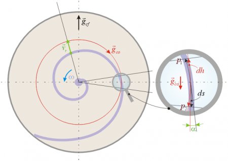
Fig 3.

For more exact analysis let us examine a very small segment of the rotating spiral duct as magnified on  fig 3. If the segment is enough short then we can consider it as a straight duct piece of length ds. There is a small angle a between the tangents of the duct and the circle that cuts the segment in its center. The effective ‘height’ dh of the liquid column in the examined segment is the length of the ds segment’s projection on the red circle. This is analogous to the situation when a slanted pipe is present in gravitational field, and the effective height of the liquid column that will determine the pressure at the bottom is the projection of the slanted pipe’s length on a vertical line (that is parallel with the gravitational force vector). The infinitesimal Coriolis pressure increase can be calculated as:

If one knows the equation of the examined spiral then it is possible to integrate these infinitesimal pressure differences and get the equation of the Coriolis pressure in the duct as the function of the angle or radius.

It is obvious that if there is a nozzle at the periphery of the rotating spiral duct and the liquid flows towards the nozzle then the relative velocity of the liquid will have a radial v_r component, that will create a Coriolis pressure gradient. This will create a pressure component that will increase in circular direction (opposite to the rotation) towards the nozzle, and it will be superposed upon the centrifugal pressure component that also increases towards the periphery. The resultant pressure at the nozzle that will determine the relative exit velocity of the liquid stream (and the resulting reaction force and torque) will be the sum of the centrifugal- and Coriolis pressure components p=p_cf+p_co.

In the case of the above analyzed lawn sprinkler with straight arms the Coriolis force had a negative effect on the energy balance because it braked the rotation and it did not increase the pressure at the nozzle; but still we have got back as much energy from the system as much we have invested. If instead of straight ducts we use spiral ducts, then we have seen that besides the normal centrifugal pressure present in the straight sprinkler we get an additional Coriolis pressure component at the nozzle. This increased pressure will create faster liquid stream at the exit of the nozzle (compared to the straight sprinkler) and produce an increased driving torque and excess energy. The source of excess energy is not only the increased driving torque, but also the increased velocity and kinetic energy of the exit stream compared to the straight-armed case.

If the exit stream is collected with appropriate geometry and its kinetic energy is partially converted into pressure energy and fed back to the pump, then a positive feedback can be established. This way even the otherwise lost (into heat) kinetic energy of the stream can be recycled and converted into additional driving torque and mechanical power. Then the pressure at the inlet of the pump will continuously increase until the regulation does not establishes an equilibrium.

An attempt to confirm the principle with CFD analysis

Today there are very powerful CFD (Computational Fluid Dynamics) programs that are claimed to be capable of modeling the physical reality with good accuracy. But this is true only for the cases where the law of energy conservation is not violated. It was a natural idea that one should try to detect the discussed additional Coriolis pressure as the source of excess energy in a rotating spiral duct using an advanced CFD software. This approach would be faster, cheaper, and offer easier evaluation than building the device in reality and performing measurements.

Fig 4.

The analyzed spiral centrifuge is shown on   fig 4 and it is made of a pipe of circular cross section having a diameter of 10 mm with a 20 mm long nozzle extension at the periphery that has an outlet opening of 5.09 mm diameter. The radial distance of the nozzle’s centerline from the axis of rotation (at the center of the spiral) is R=200 mm. The duct is assumed to be friction less (without resistance and it produces no pressure drop) and rotating in counter clockwise direction with w =628 rad/s (~6000 RPM). The fluid is water (r =997 kg/m³) at temperature of 25 C and the flow type is turbulent. The boundary conditions are: inlet velocity 50 m/s normal to the boundary, and a constant pressure of 0 Pa at the outlet of the nozzle. A symmetry plane has been used and one half of the geometry had a mesh with 1188411 finite volumes with inflated layers near the wall boundary that is a good resolution. The solver was run until the worst RMS residual was below 4.2E-06 that means a fairly good accuracy.

The aim of this run was to detect whether there is indeed a greater pressure at the inlet of the nozzle than what is expected from the centrifugal pressure; and if yes, then whether the excess pressure has a magnitude that is expected from the Coriolis pressure using the already discussed reasoning. The CFD analysis produced a solution with a pressure distribution shown on fig 5. A custom pressure range has been chosen for this picture so that the lowest displayed pressure of 9.416E6 Pa is present at the inlet of the spiral duct (dark blue color), and the highest pressure is 1.801E7 Pa at the inlet of the nozzle (red color). A small portion at the end of the nozzle is colorless because the pressure there is lower than the specified lowest displayed pressure, and it has no significance for this analysis.

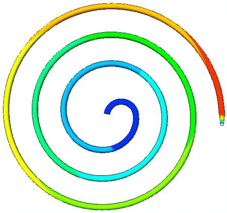
Fig 5. Pressure distribution: from 9.416E6 Pa (dark blue) - to 1.801E7 Pa (red)

The average pressure at the inlet of the spiral duct is 9.634E6 Pa that corresponds to the pressure of the external pump p₀ in our analysis. If we subtract this pressure from the highest pressure of 1.801E7 Pa at the periphery then we get the total pressure increase that supposed to be the sum of the centrifugal- and Coriolis pressure components, and it is Dp=8.376E6 Pa. The expected pressure increase due to the centrifugal pressure gradient can be calculated as p_cf=r w ²R²/2=7.864E6 Pa.

The indicated Dp pressure increase is greater than this calculated centrifugal pressure, thus an additional pressure component is indeed detected. The Coriolis pressure component supposed to be the difference between the total pressure increase Dp and the centrifugal pressure component p_cf and it is p_co=Dp - p_cf =5.12E5 Pa. Now let us try to estimate the expected Coriolis pressure for this case using the earlier discussed formulas and methodology, and compare it with the last result indicated by the CFD solution.

First of all we have to find the radial velocity of the water in the spiral pipe. This can be checked using a ZX section plane through the spiral duct, and looking for the velocity component in X direction. The radial velocity v_r changes from about 6 m/s in the first turn on the left side to about 2 m/s in the 3^rd turn on the left side of the above figure. For the sake of demonstration let us calculate with the lowest value of v_r=2 m/s. The length of the spiral pipe’s center line is 2.361 m and this does not include the length of the nozzle, nor the small semicircle shaped pipe segment that connects the spiral shape to the axis of rotation. The pitch of the spiral is fairly small thus the angle between the spiral and the circles around the axis of rotation a is small, and the length of the spiral segment’s ds projection on the circles dh will be just a little smaller ( fig 3). For the sake of simplicity let as take the total projected effective height of the water column in the circular Coriolis field of acceleration to be h=2 m (instead of 2.361 m). Now we have all the necessary parameters for the calculation of an approximate value of the expected Coriolis pressure increase at the periphery.

It can be calculated as p_co~2r v_rw h=2*997*2*628*2=5.009E6 Pa. Naturally this is only an approximation and the exact value can be calculated only by performing the integration discussed in connection with   fig 3, but it is enough good to see the expected order of magnitude. If we compare this expected 5.009E6 Pa with the 5.12E5 Pa indicated by the CFD analysis, then we see that the CFD model shows about 10 times smaller Coriolis pressure increase than what we would expect by assuming the lowest radial velocity v_r and a modest effective liquid column height h in the circular Coriolis field of acceleration. This is too big difference and it indicates that either the here presented calculation method for the pressure increase due to Coriolis pressure gradient is incorrect, or the CFD program produces wrong results for such cases (because they give correct results only when the law of energy conservation is satisfied).

There is one more weird thing in the CFD solution that confirms our suspicion about its invalidity. Namely the walls were declared to be adiabatic (that means no heat energy can pass through the walls) and a model was specified which takes into account the heat dissipation and heat conduction within the fluid. The solver was stopped only after the RMS residual of the energy equations went below 1.3E-06 that supposed to give an accurate solution. The temperature distribution of the solution is displayed on   fig 6, where the temperature at the inlet is 25 C (red) that seems to cool down to 18.9 C (dark blue) and then it heats up again to 23.3 C (yellow) at the outlet. Since the program obviously does not contain any physical model that would allow the heat energy of the liquid to be converted into any other type of energy (decreasing entropy), and since the heat can not escape through the pipe walls, it is absurd that the water seems to cool down in the solution and then it warms up again. In our adiabatic pipes we can expect some temperature increase due to internal friction within the fluid, but there is no reasonable explanation for the displayed temperature loss. This weird phenomenon indicates that the program tries to keep the law of energy conservation valid by all means even when excess energy appears, and therefore it attempts to counter balance this excess energy by ‘cooling down’ the liquid.

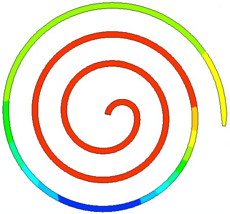
Fig 6. Temperature distribution: from 18.9 C (dark blue) to 25 C (red)

The same CFD setup was run again but taking the flow to be laminar (that is unrealistic). The laminar case produced almost the same pressure distribution because the walls of the duct were taken to be frictionless.

Conclusion

The expected Coriolis pressure p_co~5.009E6 Pa has the same order of magnitude as the centrifugal pressure p_cf=7.864E6 Pa and if we would not take the smallest value for the radial velocity but a more realistic average (or perform the exact integration), then both pressure components could have nearly the same values. That means, if the velocity of the water stream is to be unchanged then a much less external pump pressure p₀ and input power would be enough to produce the same torque and output power that follows from this exit stream velocity. On the other hand if the p₀ is kept unchanged then the stream velocity, the driving torque, and the output power would increase due to the Coriolis pressure. The Coriolis pressure component produces excess energy.

The phenomenon can be summarized in the following manner:

When a liquid is present in a rotating frame of reference and it moves from the axis of rotation towards the nozzle at the periphery, then the liquid will exert a negative retarding Coriolis torque on the rotating platform and counteract the positive effect of the centrifugal pressure. This energy loss will balance the energy gain of the liquid caused by the centrifugal pressure. This happened in the case of the straight-armed lawn sprinkler.

But if in a rotating frame of reference the liquid is allowed to flow towards the periphery in a spiral duct (opposite to the direction of rotation) so that a Coriolis pressure component is allowed to increase towards the exit nozzle, then this Coriolis pressure will increase the energy of the liquid just like the centrifugal pressure, while there is no other effect that could counteract the excess energy from this pressure gain. This lack of symmetry, or the violation of ‘action and reaction’ is the source of excess energy. (In the sense that ex. the centrifugal pressure is the energy increasing positive ‘action’, and the retarding Coriolis torque is the corresponding negative ‘reaction’ keeping the law of energy conservation valid. While the energy increasing positive ‘action’ of the Coriolis pressure has no corresponding negative ‘reaction’ that could keep the law of energy conservation valid).

The commercial CFD programs are designed to always comply with the law of energy conservation, thus we can not expect that they should correctly model a situation when the same law must be violated due to the Coriolis pressure. Therefore they can be only of limited use for such research, ex. to analyze cases when the law of energy conservation is not violated. This research either requires that special CFD code should be written that would correctly model the Coriolis pressure increase, or even better to build practical devices and perform accurate measurements.

Practical considerations and application of the principle

We have analyzed so far only ideal cases where the friction resistance of the ducts were neglected and consequently there was no pressure drop in the ducts. It is much easier to detect a possible energy gain in such idealized systems than in realistic situations including friction losses. If one finds excess energy in an ideal case then it will be present more or less in real cases too. Unfortunately in practice there is always some friction resistance and head loss, especially in such thin and long pipes as in our last example, particularly when the flow is turbulent.

In order to check the magnitude of the head loss due to friction resistance, the same spiral pipe has been analyzed with the CFD program that is shown on  fig 4, but taking the friction resistance into account while the spiral is stationary. The inlet water velocity was 50 m/s and the pressure at the outlet of the nozzle was taken to be 0 Pa just as in previous case. The solution of this CFD analysis showed an inlet pressure of 2.2E7 Pa while the pressure at the inlet of the nozzle was 1.744E7 Pa. The difference of these two pressures p_f=4.56E6 Pa is the pressure drop due to the friction resistance of the pipe. If we compare this with the estimated Coriolis pressure p_co~5.009E6 Pa then we can see that they are almost the same, and the positive effect of the Coriolis pressure can be lost in practical devices if the friction resistance of the ducts are too high.

In practical designs the friction resistance of the ducts should be minimized, that might require using shorter ducts with increased cross section area, and made of special smooth materials. The number of turns and the pitch of the spiral requires also optimization. If the pitch is higher, then the radial velocity is higher, but the effective liquid column height h in the Coriolis field of acceleration will be shorter.

If the aim is to recycle the kinetic energy of the exit liquid stream, then one good solution could be that instead of separate spiral pipes, a drum-like design is used with spirally arranged guiding walls within the drum. The liquid could flow on spiral trajectories between the guiding walls towards special nozzles at the periphery. The cross section area of the nozzles would diminish towards the exit opening, not as the result of the spiral guiding walls coming closer together, but as the result of slanted disc sidewalls. The thin exit openings of these nozzles could cover the whole outer circumference of the (saucer shaped) drum, so that only the ends of the guiding walls would separate one nozzle exit from the other. This way the continuous quasi tangential water stream could be collected in a surrounding stationary duct and lead the water back to the pump while lowering its velocity and increasing its pressure. The US patent 4357797 of Siptrott Fred M can also give some ideas how to recycle the kinetic energy of the exit stream, convert it to pressure, and feed it back to the pump (even if his claims about his device are incorrect).

The Coriolis pressure as the source of excess energy in imploding liquid flows

The same principle is valid not only in rotating systems with ‘exploding’ flow types (when the liquid flows from the axis towards the periphery), but also with ‘imploding’ flow types (when the flow is directed from the periphery towards the axis of rotation). Even in imploding flows the fluid should follow a spiral trajectory with the difference that the relative tangential velocity component of the flow has the same direction as the rotation of the ducts. In such case the Coriolis field of acceleration has the same direction as the rotation, and the Coriolis pressure increases towards the axis. With appropriate designs - even if the spiral flow develops without using separate ducts - this additional Coriolis pressure gradient can be converted into increasing fluid velocity (like with funnel shaped outer walls in which imploding helical flow develops). Such natural helical imploding flows can be observed in nature as vortexes, whirlpools and hurricanes.

Zoltan Losonc

Appendix:

The pressure in a centrifuge

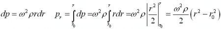
Where: p – pressure; ρ - density of the fluid; ω - angular velocity; S – surface area; dV – elementary volume; dm – the mass of the fluid within dV; a – acceleration, F – force;   r–radius.

We have assumed that ω is constant and the fluid is homogenous and incompressible. The pressure is the same whether we have only a segment of the rotating drum or the whole drum, and it does not depend on the shape of the segment. return